Anomaly Detection Using Standard and Poor's 500 Index
Detecting anomalies around S&P-500 using LSTM AutoEncoders.
This is implementation of Anomaly Detection using Time series data in Keras API. Specifically, designing and training and
LSTM autoencoder using the Keras API with Tensorflow 2 as the backend to detect anomalies (sudden price changes) in the S&P 500 index.
The complete code for the project can be found here.
Data Set Summary & Exploration
We have used S&P 500, or simply the S&P, as the time series data which is a, stock market index that measures the stock performance of 500 large companies listed on stock exchanges in the United States. It is one of the most commonly followed equity indices. Anomaly Detection would be used to measure abrupt changes in the stock prices of S&P 500 newplot. The S&P 500 index data is in the form of a csv file. The data is further processed into train and test data
- The size of training set is 6523.
- The size of test set is 1639.
- The number of unique classes/labels in the data set is 2 ie. date and close.
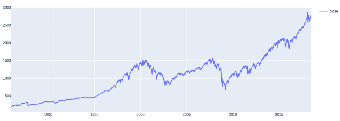
The dataset is in csv format with date and close price from 1986 to 2018.
Here is the exploratory visualisation of the dataset. Here is the graph of dataset.
Data preprocessing
The csv data was further processed into training data and test data using pandas. Here 80% of dataframe will be used for training and
20% will be used for testing. We use iloc method to specify slicing by index.
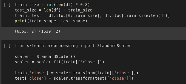
The target vector is standarized by removing the mean and scaling it to the unit variance
using StandardScaler function from sklearn.preprocessing
The Data vectors are then reshaped in the form n(samples)
by n(time_steps) by n(features) in line with Time-Series modelling.
Create Test and Train Data
Segregate the data in a sliding-window of 30 days per partition.Then, Save each partition of 30 days as an element in the training vector. Add the following day's closing value as a corresponding element in the target vector.
Model Architecture & Training
Model used for anomaly detection is made using LSTM architecture and then the autoencoder is trained. The entire process is further explained below.
LSTM Architecture Autoencoder
First let's understand the meaning of LSTM architecture.
LSTM stands for Long Short-term Memory, which is also an artificial neural network similar to Recurrent Neural Network(RNN). It processes the datas passing on the information as it propagates. It has a cell, allows the neural network to keep or forget the information.
For this, an LSTM Autoencoder network is built which visualises the architecture and data flow. So here’s how anomalies using an autoencoder is gonna get detected. First, the data is trained with no anomalies and then take the new data point and try to reconstruct that using an autoencoder. If the reconstruction error for the new dataset is above some threshold, then it's going to label that example/data point as an anomaly.
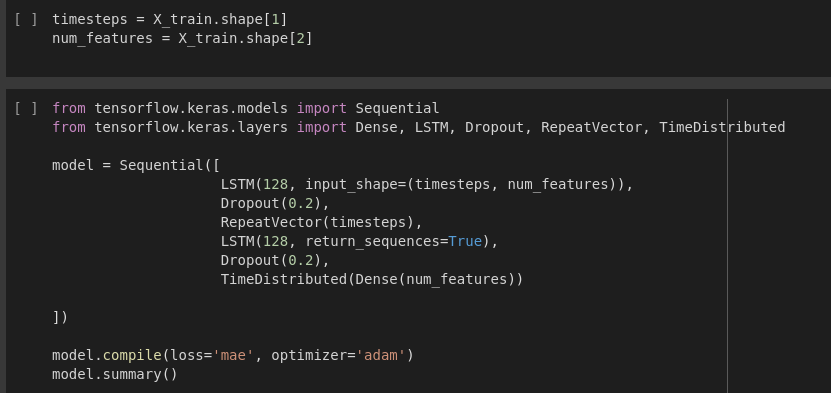
In the above codes, X_train array i.e. (6523, 30, 1) is assigned. While building the LSTM architecture, Sequential model from keras API is used. The sample data is 1% which is 2D array and is passed to LSTM as input. The output of the layer is going to be a feature vector of input data. One LSTM layer is created with the number of cells to be 128. Input shape is equal to no. of time_stpes divided by no. of features. Then, the Dropout regularization is added to 0.2. Since the network is LSTM, we need to duplicate this vector using RepeatVector. It’s purpose is to just replicate the feature vector from the output of LSTM layer 3o times. The encoder is done here.
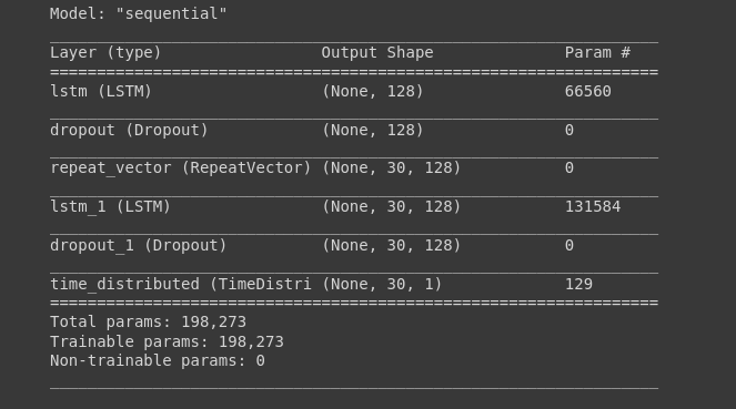
In decoder layer, TimeDistributed function creates a dense layer with number of nodes equal to the number of features. And the model is compiled finally using adam optimizer function which is gradient descent optimizer.The model summary is shown above.
Autoencoder Training
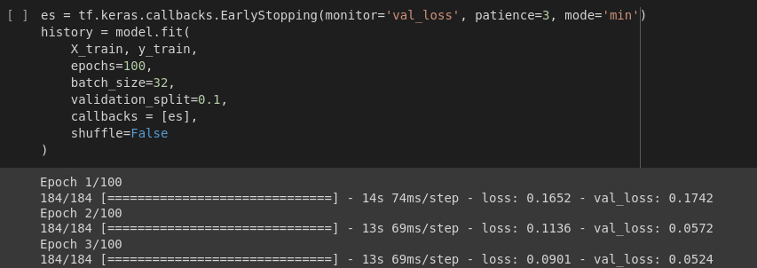
Keras Callback is created using early stopping so that the number of epochs are not needed to hard code. If the network doesn’t improve for 3 consecutive epochs,i.e. validation loss is not decreased we are going to stop our training process.
That is the meaning of patience. And now let’s fit the model to our calling data. No. of epochs is set to high as higher the epochs, more the accuracy of training. 10 % of the data is set for validation. And then the callback is done using es i.e.
EarlyStopping.
Plot Metrics and Evaluate the Model
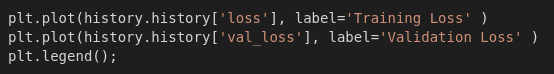
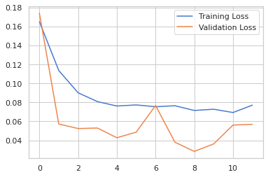
Now the matrix that is training loss and validation loss is plotted using matplotlib. In the plot, validation loss is consistently found to be lower than training loss that means the training data due to the high dropout value we used So you can change the hyperparameters in 5th step to optimize the model.
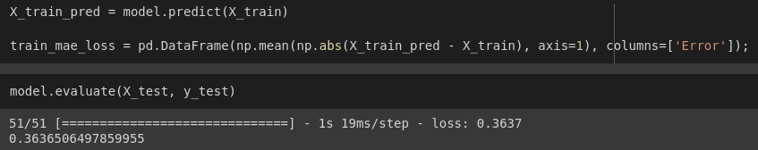
We need to still predict the anomaly in our test data by calculating the mean absolute error on the training data. First, let’s get prediction on our training data. And then we evaluate the model on our test data.
Then distribution loss of training mean absolute error is shown using seaborn.
![]()
That shows the output like:
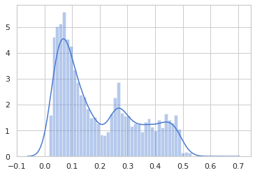
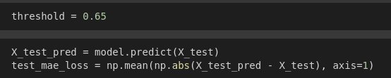
Here, we can set the threshold as 0.65 as no value is larger than that. Now, let’s calculate the mean absolute error on test set in similar way to the training set and then plot the distribution loss.
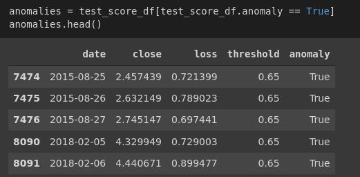
Detect anomalies in S&P-500 data
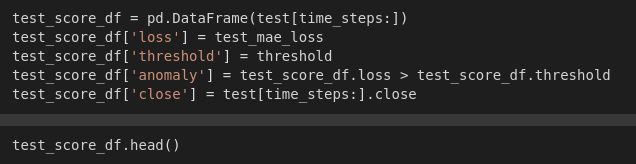
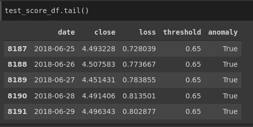
Now let's build a data frame containing loss and anomalies values. Then let’s create a boolean-valued column called an anomaly, to track whether the input in that corresponding row is an anomaly or not using the condition that the loss is greater than the threshold or not. Lastly, we will track the closing price
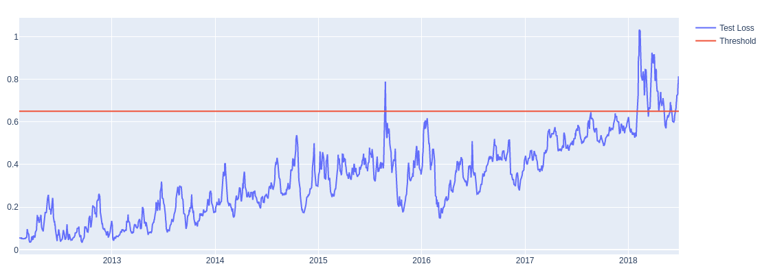
Now let’s plot train and test loss value and overlay the line for threshold. First, we will create an empty figure and then use add_trace() method to populate the figure. We are going to create line plot using go.Scatter() method
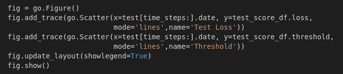
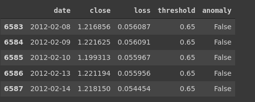
This shows result like this
This is the anomaly test score:
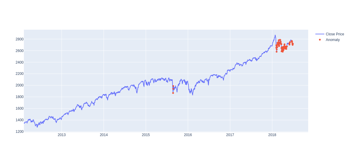
The closing price and the anomaly graph is plotted as shown as below:
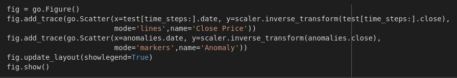
The output with orange anomalies and blue closing price is shown below:
Thanks for reading!